Data Validation In Microsoft excel

Ever been hounded by the thought of data entry errors. Simple Mistakes and even plain simple mistakes can wreck havoc on the data analysis.

If you have a defined number of options to choose from and enter then the data validation option comes to the rescue.

Example:

Entering the Date, Month and Year in 3 different Columns.

Date: Can be made to choose from 1-31

Month: Can be made to choose from Jan-Dec

Year: Any logical defined Range can be Taken.


How To:

Navigate to the Data Tab>Data Validation

Thats it. This way you restrict users to select values between the defined range only.

There are a number of other options also.

Please ping me for any specific details you might require.

Thanks Again.

Coolest Budget Vs Actual Chart

Hi,

Will share with you the coolest thing I have learnt recently in Charting.

The entire write up is not yet completed, will do that that surely by Sunday.

Excel Shortcuts

Living with Excel Shortcuts

These are the Shortcuts that I use often and saves a lot of time for me.

1. ( Ctrl + * ) allows us to select the current range until the end of the data set is hit.

2. ( Shift + F10 ) – We often need to use the right click menu and using a mouse is cumbersome. This one does the trick.

3. (Ctrl + Page Down) & ( Ctrl + Page Up) – Quickly move between worksheets in a workbook.

4. ( F5 & Alt + S) to open up the Goto Special Menu.

5. (Ctrl + Shift + L) – Turn the filters on and off.

Goal Seek In Excel - An example

Hello friends , today we will discuss the Goal Seek Function. This function allows us to alter data in formulas to get different results or results that we require. We can then compare results as per our requirement.

Lets take an example.

Everyone retires and we need to plan for it. Why not do it from excel.

Lets suppose I want Rs. 1,00,000,00 at age 50 (Please don't ask what i am going to use that for). Currently I am 30 ( That's True). We will be using the future Value formula in excel to determine the time value of money. 

Now lets assume the following variables.

Interest Rate –                      8 % P/Annum

Frequency of Compounding -  Monthly

Remaining No of Years -         20

We also assume that the payments are made at the beginning of the month.

Once we have entered the Data as highlighted in Yellow as per our requirement.

Go to the data Tab in Excel and Select "What if Analysis". Then Goto the goal Seek function from the drop down and click Ok.

The below Screen will open up.

Now I hope the diagram is Self Explanatory.

We have to set cell C3 to the required value (1,00,000,00) and click ok, and Amen. You will need to invest Rs. 16,865 per month to retire with Rs.1 Crore in 20 years. Too long a wait but now you at least know it. There are other variations too to this function and will be discussed in the coming posts.

Thanks for visiting as always.

Signing Off

Please comment for any queries that you may have.

Paste Operations - Part II

PART 2: PASTE OPERATIONS

Paste option also comes with a handful of operations. We can Add, Subtract, Multiply and Divide while pasting a set of values. An example will illustrate it better.

A Sales Department has the following weekly sales data.

Now for instance the department manager has done an error in the quantity and the pricing on all days of the week. The below is the difference data.

Now the original data needs to be corrected. We just have to copy the error data ( quantity and price and paste in over the original data using paste special (Addition Option). The same could to done to multiple, divide or Subtract.

Shortcut Key:  

Add :      After Ctrl + C , Press Alt + E followed by S & D

Multiply:    After Ctrl + C , Press Alt + E followed by S & M

Divide:      After Ctrl + C , Press Alt + E followed by S & I

Subtract:  After Ctrl + C , Press Alt + E followed by S & S

Please post your feedback or any Queries.

Humble Copy Amazing Paste

Its Copy Paste Again. To me a Nobel should be awarded to the one to introduced the idea of copy paste. The Greatest gift to the dead on the deadline professional. We have all done it and will do it till our last breath, then Why not familiarize ourselves with a few amazing things that could be done through this humble yet life saving tool.

We will deal with this in three parts :

1. Paste Options ,  2. Operations while Pasting,  3. Pasting differently

The below is the paste special screen. 

PART 1: PASTE OPTIONS

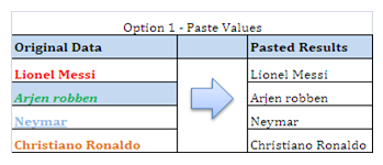
Values: 

This option copies only the value in the cell or range leaving behind the formats/formulas . Actually this is what happens when we take footballers from Club football to Fifa. They loose 

everything they have.

 

Formulas: This copies the formulas in the source cells to the destination.

Suppose we want to copy the % calculation from Tom’s Score card to Harry’s. This option is useful then. It can also be done with a simple copy paste but the formats also get copied that way. You can also drag the handle if the cells are adjacent.

Shortcut Key: After Ctrl + C , Press Alt + E followed by S & F

Formats: We are talking only formats here. The below example will illustrate that.

Now we want to copy the formats to the destination without touching the data. Paste Formats is at the rescue.

Shortcut Key: After Ctrl + C , Press Alt + E followed by S & T

Comments: Copying comments only from one cell to another.

I have copied the comments from Messi to Ronaldo. Both are great players to me.:)

Shortcut Key: After Ctrl + C , Press Alt + E followed by S & C

Validations: we have created a cell validation list as below and want to copy it to another cell . Note we do not want to copy the already selected option.

Shortcut Key: After Ctrl + C , Press Alt + E followed by S & N.

Column Width: Now we have the below two sets of data and we want to have the same column widths in harry as in Tom’s Data. This could be achieved by using the column widths option.

You Might ask what about The Row Heights, Can we not copy that ?? Sorry friends that needs a VBA Solution and I am not an expert at it, but I can still provide you with a solution if needed. Just Ask. 

Shortcut Key: After Ctrl + C , Press Alt + E followed by S & W

There are also other options available that could mix and match the requirements as below where the names are self explanatory.

1. All Using Source Theme

2. All except Borders

3. Formulas and Numbers formats.

4. Values and Number formats.

I will be following up this one with part 2 & 3 very very shortly.

Hope you liked this small piece of information. Please post your queries and I assure a reply within 24 hours.

Signing off.

Nishant